

By Aditi Goyal, Genetics & Genomics, Statistics ‘22
Author’s Note: As the field of computational biology grows, machine learning continues to have larger impacts in research, genomics research in particular. Genetic algorithms are an incredible example of how computer science and biology work hand in hand and can provide us with information that would otherwise take decades to obtain. I was inspired to write a review overviewing genetic algorithms and their impact on biology research after reading a news article about them. This paper is not intended to serve as a tutorial of any kind when it comes to writing a genetic algorithm. Rather, it serves to introduce this concept to someone with little to no background in computer science or bioinformatics.
Introduction
In 2008, Antoine Danchin wrote that “there is more than a crude metaphor behind the analogy between cells and computers.” [1] He also stated that the “genetic program is more than a metaphor and that cells, bacteria, in particular, are Turing machines.” [1] This is the fundamental theory that has been the basis of systems biology and has inspired the development of genetic algorithms. Genetic algorithms (GAs) provide a method to model evolution. They are based on Darwin’s theory of evolution, and computationally create the conditions of natural selection. Using genetic algorithms, one can track the progression of a certain gene or chromosome throughout multiple generations. In this paper, we discuss the components of a genetic algorithm, and how they can be modified and applied for various biological studies.
Background
GA’s are an example of a metaheuristic algorithm that is designed to find solutions to NP-hard problems [2, 3]. NP problems, aka Non-deterministic Polynomial-time problems, describe optimization problems that take a polynomial amount of time to solve via a brute force method. This is best understood through an example, the most classic one being the Traveling Salesman Problem [4]. If a salesman has to travel to five different locations, how should he pick the order of his destinations, in order to minimize the distance he travels? The solution to this problem is to calculate the total distance for each combination and pick the shortest route. At five destinations alone, there are 120 possible routes to consider. Naturally, as the number of ‘destinations’ increases, the number of possible routes will increase, as will the time it takes to calculate all options. In more complicated scenarios, such as an evolution prediction system, this problem becomes exponentially more difficult to solve, and therefore requires optimization.
GA’s are “problem independent” optimization algorithms [2, 3]. This means that the parameterization of the algorithm does not depend on any certain situation, and can be modified by the user depending on the situation. This class of optimization algorithms is often referred to as a metaheuristic algorithm. The key idea is that these types of optimization functions trade accuracy for efficiency. Essentially, they aim to approximate a solution using the least amount of time and computing power, as opposed to providing a high degree of accuracy that may take significantly more resources.
Components of a Genetic Algorithm
There are only two components essential to creating a GA: a population, and a fitness function [I*]. These two factors are sufficient to create the skeleton of a GA. Withal, most GA’s are modeled after Darwin’s theory of evolution [j*]. They use the components of fitness, inheritance, and natural variation through recombination and mutation to model how a genetic lineage will change and adapt over time [j*]. Therefore, these components must also be incorporated into the GA in order to more accurately mimic natural selection.
Population
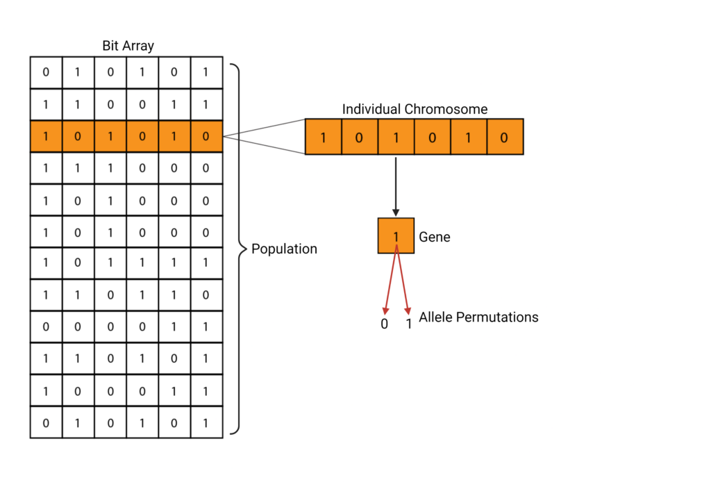
A population is defined using the first generation, or F1. This can be a set of genes, chromosomes, or other units of interest [7]. This generation can be represented in several ways, but the most common technique is to use a bit array where different permutations of 0’s and 1’s represent different genes [7].
Selection & Fitness Functions
Now that a population has been initialized, it needs to undergo selection. During selection, the algorithm needs to select which individuals from the population will be continuing onto the next generation. This is done through the fitness function [3]. The fitness function aims to parameterize the survival of a certain individual within the population and provide a fitness score. This accounts for the fitness of each genetic trait and then computes the probability that the trait in question will continue onwards. The fitness score can be represented in different ways. A common method is using a binary system. For example, consider a chromosome being defined as a set of bits (see Figure 1). A neutral, or wild-type allele can be represented with a zero. A beneficial allele or one that confers some sort of advantage over the wild-type is represented using a 1. The fitness function would then be defined to calculate the fitness of each chromosome. In this example, the fitness is equivalent to the sum of the binary scores.
Chromosomes with a higher fitness score represent chromosomes that have more beneficial traits as compared to chromosomes with lower fitness scores. Therefore, chromosomes that maximize the fitness score will be preferred.
Inheritance & Genetic Variation
The fittest individuals are then propagated onwards to the “breeding” phase, while only a small proportion of the fewer fit individuals are carried forward. This is the step that mimics “natural selection”, as we are selecting for the more fit individuals, and only a small proportion of the fewer fit individuals are surviving due to chance.
Now that the survivors have been identified, we can use GA operators to create the next generation. GA operators are how genetic variation is modeled [7]. As such, the two most common operators in any GA are mutation rates and recombination patterns. The F2 generation is created by pairing two individuals from F1 at random and using our operators to create a unique F2.
Mutations are commonly represented using bit changes [3]. Because our original population was defined in binary, our mutation probability function represents the probability of a bit switch, i.e. the probability that a 0 would switch to a 1, or vice versa. These probabilities are usually quite low and have a minor impact on the genetic variation.
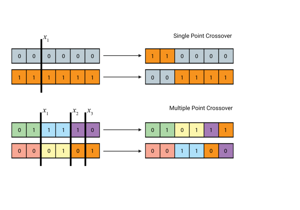
Recombination, or crossovers, is where the majority of new genetic variations arise. These are modeled by choosing a point of recombination, and essentially swapping bit strings at that point. A simple GA uses a single point crossover, where only one crossover occurs per chromosome. However, a GA can easily be adapted to have multiple crossover points [8, 9].
On average, via the mutation and crossover operators, the fitness level of F2 should be higher than F1. By carrying some of the fewer fit individuals, we allow for a larger gene pool and therefore allow for more possibilities for genetic combinations, but the gene pool should be predominated by favorable genes [3].
Termination
This three-step pattern of selection, variation, and propagation is repeated until a certain threshold is reached. This threshold can be a variety of factors, ranging anywhere from a preset number of generations to a certain average fitness level. Typically, termination occurs when population convergence occurs, meaning that the offspring generation is not significantly better than the generation before it [10].
Modifications to GA’s
As one can see, this is a rather simplistic approach to evolution. There are several biological factors that remain unaddressed in a three-step process. Consequently, there are many ways to expand a GA to more closely resemble the complexity of natural evolution. The following section shall briefly overview a few of the different techniques used in tandem with a GA to add further resolution to this prediction process.
Speciation
A GA can be combined with a speciation heuristic that discourages crossover pairs between two individuals that are very similar, allowing for more diverse offspring generations [11, 12]. Without this speciation parameter, early convergence is a likely possibility [12]. Early convergence describes the event that the ideal individual, i.e. the individual with the optimized fitness score, is reached in too few generations.
Elitism
Elitism is a commonly used approach to ensure that the fitness level will never decrease from one generation to the next [13]. Elitism describes the decision to carry on the highest-rated individuals from one generation to the next with no change [13, 14]. Elitism also ensures that genetic information is not lost. Since each offspring must be ‘equal or better’ than the generation before it, it is guaranteed that the parental genotypes will carry through generations, changing at a much slower rate than a pure GA would model [15].
Adaptive Genetic Algorithms
Adaptive Genetic Algorithms (AGA’s) are a burgeoning subfield of GA development. An AGA will continuously modify the mutation and crossover operators in order to maintain population diversity, while also keeping the convergence rate consistent [16]. This is computationally expensive but often produces more realistic results, especially when calculating the time it would take to reach the optimal fitness. The Mahmoodabadi et al team compared AGA’s to 3 other optimization functions and found that “AGA offers the highest accuracy and the best performance on most unimodal and multimodal test functions” [17].
Interactive Genetic Algorithms
As previously stated, the fitness function is critical to creating a GA. However, there arise several instances where a fitness function cannot be accurately defined. This is particularly true for species that have elaborate mating rituals, as that is a form of selection that would be computationally expensive to recreate. In these situations, one can use an interactive genetic algorithm (IGA). IGA’s operate in a similar fashion to GA’s, but they require user input at the fitness calculation point.
While this method does provide some way of modeling a population without having a predefined fitness function, it has glaring drawbacks. Primarily, this process is not feasible for large populations, as it puts the burden of calculating the fitness on the user, and it also leaves room for subjective bias from the user. However, this subjective component been viewed as an advantage in several fields, particularly the fashion industry [18]. Designers have been investigating IGA’s as a method to generate new styles, as the algorithm depends on user validation of what is considered to be a good design versus a bad one [18].
Applications
Genetic algorithms have a far-reaching effect on computational efforts in every field, especially in biology. As the name suggests, genetic algorithms have a huge impact on evolutionary biology, as they can assist with phylogeny construction for unrooted trees [19]. Oftentimes, evolutionary data sets are incomplete. This can result in billions of potential unrooted phylogenetic trees. As the Hill et al team describes, “for only 13 taxa, there are more than 13 billion possible unrooted phylogenetic trees,” [19].
Testing each of these combinations and determining the best fit is yet another example of an optimization problem– one which a GA can easily crack. Hill et al applied a GA to a set of amino acid sequences and built a phylogenetic tree comparing protein similarities [19]. They found that a program called Phanto, “infers the phylogeny of 92 taxa with 533 amino acids, including gaps in a little over half an hour using a regular desktop PC” [19].
Similarly, the Wong et al team tackled the infamous protein folding prediction problem using GA’s [20]. They used the HP Lattice model to simplify a protein structure and used the iterative nature of a GA to find a configuration that minimized the energy required to fold a protein into that shape. The HP Lattice model stands for Hydrophobic Polar Lattice and seeks to model the hydrophobicity interactions that occur between different amino acid residues in the secondary structure of a protein [20]. They found that a GA performed better than some of the newer protein folding predictive programs available today [20].
GA’s are an incredible tool for cancer research as well. The Mitra et al team used a GA to study bladder cancer [21]. They conducted quantitative PCR on tissue samples from 65 patients and identified 70 genes of interest. Of these 70 genes, three genes in particular, were identified in a novel pathway. They discovered that ICAM1 was up-regulated relative to MAP2K6, while MAP2K6 was up-regulated relative to KDR. This pathway was considered to be novel because individually, all three genes displayed no signs of significant changes in regulation. By applying a GA, the Mitra team was able to identify this pattern between all three genes. Uncoincidentally, “ICAM1 and MAP2K6 are both in the ICAM1 pathway, which has been reported as being associated with cancer progression, while KDR has been reported as being associated with the vascularization supporting tumors” [21, 22, 23].
Another groundbreaking discovery was made by applying GA’s to p53 research. P53 is an essential tumor suppressor [24]. Most cancerous tumors can be attributed, in part, to a mutation in the p53 gene, making it an excellent candidate for oncology research. The Millet et al team investigated a possible p53 gene signature for breast cancer, hoping to find an accurate prediction system for the severity of breast cancer [25]. They analyzed 251 transcriptomes from patient data and found a 32 gene signature that could serve as a predictor for breast cancer severity [23, 25]. They also found that “the p53 signature could significantly distinguish patients having more or less benefit from specific systemic adjuvant therapies and locoregional radiotherapy,” [25].
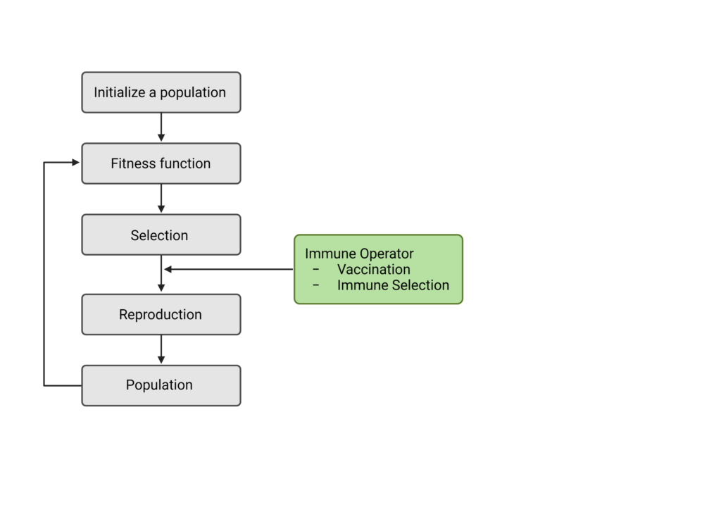
GA’s have also had a huge impact on immunology, vaccine development in particular. Licheng Jiao and Lei Wang developed a new type of GA called the Immunity Genetic Algorithm [26]. This system mimics a typical GA but adds a two-step ‘immunological’ parameter (Figure 3). Much like a GA, the fitness function is applied to a population, which then triggers mutation and crossover. However, after these steps, the program mimics ‘vaccination’ and ‘immune selection. These two steps are referred to as the “Immune Operator” [26]. They are designed to raise a genetic advantage in individuals who respond well to the vaccine and confer a disadvantage to those with a ‘weaker’ immune response. In essence, the vaccination step acts as a secondary mutation, as it is acting as an external change factor in each individual’s fitness. Similarly, the ‘immune selection’ step acts as a secondary fitness function, as it measures the immune response post-vaccine. If evolution is continuing as it should, each generation should have an improved immune response to the vaccine until convergence is reached.
Conclusion
GA’s have a broad reach in all fields of research, from fashion to immunology. Their success is due to three critical components underlying their programming: they are simple to write, easy to customize, and efficient to run. This flexibility and independence are what will allow programs like GA’s to become commonplace in research, across all disciplines. In particular, as biology research continues to merge with computer science and advanced modeling techniques, applications like GA’s have the potential to solve problems and raise questions about our world that we may have never imagined before.
References:
- Danchin, Antoine. “Bacteria as computers making computers.” FEMS microbiology reviews vol. 33,1 (2009): 3-26. doi:10.1111/j.1574-6976.2008.00137.x
- Said, Gamal Abd El-Nasser A., Abeer M. Mahmoud, and El-Sayed M. El-Horbaty. “A comparative study of meta-heuristic algorithms for solving quadratic assignment problem.” arXiv preprint arXiv:1407.4863 (2014).
- Marek Obitko, “III. Search Space.” Search Space, courses.cs.washington.edu/courses/cse473/06sp/GeneticAlgDemo/searchs.html.
- Hoffman K.L., Padberg M. (2001) Traveling salesman problem. In: Gass S.I., Harris C.M. (eds) Encyclopedia of Operations Research and Management Science. Springer, New York, NY. https://doi.org/10.1007/1-4020-0611-X_1068
- Whitley, D. A genetic algorithm tutorial. Stat Comput 4, 65–85 (1994). https://doi.org/10.1007/BF00175354
- McCall, John. “Genetic algorithms for modelling and optimisation.” Journal of computational and Applied Mathematics 184.1 (2005): 205-222.
- Carr, Jenna. An Introduction to Genetic Algorithms. Whitman University, 2014, www.whitman.edu/Documents/Academics/Mathematics/2014/carrjk.pdf.
- Hassanat, Ahmad et al. “Choosing Mutation and Crossover Ratios for Genetic Algorithms—A Review with a New Dynamic Approach.” Information 10.12 (2019): 390. Crossref. Web.
- Gupta, Isha, & Anshu Parashar. “Study of Crossover operators in Genetic Algorithm for Travelling Salesman Problem.” International Journal of Advanced Research in Computer Science [Online], 2.4 (2011): 194-198. Web. 17 May. 2021
- Alkafaween, Esra’a. (2015). Novel Methods for Enhancing the Performance of Genetic Algorithms. 10.13140/RG.2.2.21478.04163.
- Duda, J.. “Speciation, clustering and other genetic algorithm improvements for structural topology optimization.” (1996).
- Duda, J. W., and Jakiela, M. J. (March 1, 1997). “Generation and Classification of Structural Topologies With Genetic Algorithm Speciation.” ASME. J. Mech. Des. March 1997; 119(1): 127–131.
- J. A. Vasconcelos, J. A. Ramirez, R. H. C. Takahashi and R. R. Saldanha, “Improvements in genetic algorithms,” in IEEE Transactions on Magnetics, vol. 37, no. 5, pp. 3414-3417, Sept. 2001, doi: 10.1109/20.952626.
- Ishibuchi H., Tsukamoto N., Nojima Y. (2008) Examining the Effect of Elitism in Cellular Genetic Algorithms Using Two Neighborhood Structures. In: Rudolph G., Jansen T., Beume N., Lucas S., Poloni C. (eds) Parallel Problem Solving from Nature – PPSN X. PPSN 2008. Lecture Notes in Computer Science, vol 5199. Springer, Berlin, Heidelberg. https://doi.org/10.1007/978-3-540-87700-4_46
- Thierens, Dirk. Selection schemes, elitist recombination, and selection intensity. Vol. 1998. Utrecht University: Information and Computing Sciences, 1998.
- C. Lin, “An Adaptive Genetic Algorithm Based on Population Diversity Strategy,” 2009 Third International Conference on Genetic and Evolutionary Computing, 2009, pp. 93-96, doi: 10.1109/WGEC.2009.67.
- Mahmoodabadi, M. J., and A. R. Nemati. “A novel adaptive genetic algorithm for global optimization of mathematical test functions and real-world problems.” Engineering Science and Technology, an International Journal 19.4 (2016): 2002-2021.
- Cho, Sung-Bae. “Towards creative evolutionary systems with interactive genetic algorithm.” Applied Intelligence 16.2 (2002): 129-138.
- Hill, Tobias, et al. “Genetic algorithm for large-scale maximum parsimony phylogenetic analysis of proteins.” Biochimica et Biophysica Acta (BBA)-General Subjects 1725.1 (2005): 19-29.
- van Batenburg FH, Gultyaev AP, Pleij CW. An APL-programmed genetic algorithm for the prediction of RNA secondary structure. J Theor Biol. 1995 Jun 7;174(3):269-80. doi: 10.1006/jtbi.1995.0098. PMID: 7545258.
- Mitra, A.P., Almal, A.A., George, B. et al. The use of genetic programming in the analysis of quantitative gene expression profiles for identification of nodal status in bladder cancer. BMC Cancer 6, 159 (2006). https://doi.org/10.1186/1471-2407-6-159
- Hubbard AK, Rothlein R. Intercellular adhesion molecule-1 (ICAM-1) expression and cell signaling cascades. Free Radic Biol Med. 2000;28:1379–1386.
- Worzel, William P et al. “Applications of genetic programming in cancer research.” The international journal of biochemistry & cell biology vol. 41,2 (2009): 405-13. doi:10.1016/j.biocel.2008.09.025
- National Center for Biotechnology Information (US). Genes and Disease [Internet]. Bethesda (MD): National Center for Biotechnology Information (US); 1998-. The p53 tumor suppressor protein. Available from: https://www.ncbi.nlm.nih.gov/books/NBK22268/
- Miller LD, Smeds J, Joshy G, Vega VB, Vergara L, Ploner A, Pawitan Y, Hall P, Klaar S, Liu ET, Bergh J. An expression signature for p53 status in human breast cancer predicts mutation status, transcriptional effects, and patient survival. Proceedings of the National Academy of Sciences. 2005 Sep 20;102(38):13550–5.
- Jiao, Licheng, and Lei Wang. “A novel genetic algorithm based on immunity.” IEEE Transactions on Systems, Man, and Cybernetics-part A: systems and humans 30.5 (2000): 552-561.